HardWACC: Building an HLS tool from scratch

Introduction

At Imperial College London, second-year computing students tackle 3 big group projects: PintOS, WACC, and DRP. Each of these projects focus on developing different skills needed by a software engineer. WACC is a project where you make a compiler from scratch, and unlike the previous project (PintOS), you don’t have any skeleton or framework code to guide you. The specification is quite clear on what you have to do: write a compiler that compiles the WACC programming language. Other than that, there are not many restrictions on how you go about this task.

Our group decided to make the most of this freedom, and explore various aspects of compiler development that took our interest. This lead to writing quite an interesting compiler, some of which we will explore today. Namely, we will be looking at these sections:

• the AST
• the typechecker
• the parts of the backend pipeline (CFGs, SSA, etc.)

and most interestingly:

• HardWACC

Overview

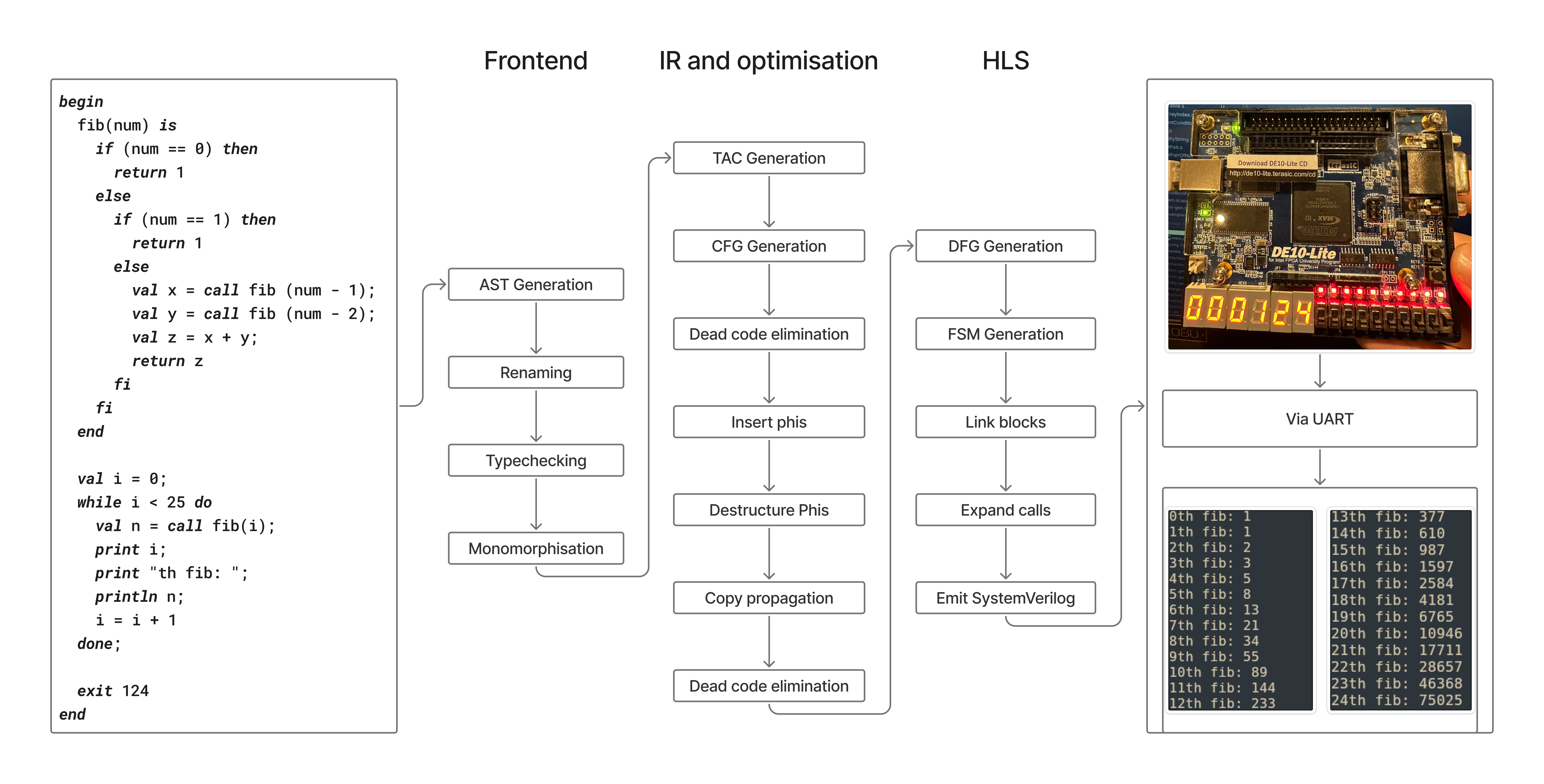
Here is an overview of the compilation pipeline.

The AST

AST design is hard - you’re constantly balancing ergonomics, reducing code duplication, and simplicity. There’s many different ways you can solve the problems, and I’m going to explain and justify how we tackled them.

Representation

Your AST needs to change between stages. Each stage of the frontend pipeline adds, removes or changes data from the previous stages. The easiest way to solve this problem is to just duplicate the entire AST ADT for each phase and change the required pieces. This however has a code duplication problem - you copy the whole AST, only making a few changes.

One way this is solved is by annotating each node type with a set of type parameters:

sealed abstract class Expr[Ident, TypeInfo, ...]
// Ident represents the type of a identifier. Before renaming, this may be a plain String, after renaming it might be an Integer
// TypeInfo represents the type of the data used to annotate nodes with type information. Before type checking, it might be Unit; afterwards, it might be SemanticType

type ParsedExpr = Expr[String, Unit, ...]
type TypecheckedExpr = Expr[RenamedIdent, SemanticType, ...]
// RenamedIdent is a ADT representing a an identifier
// SemanticType is an ADT representing a target language-level type

This works well, but a problem arises if you want to add any more type parameters. The type signature of every node becomes unweildy. A way to fix this is by leveraging type-level functions. You define a function for each piece of data of the AST you want to change the type of between stages. The domain of the function as a set of phase phantom types. The range of the function is the type of that piece of data at that stage in the frontend pipeline.

sealed abstract class Phase

// The phase type hierarchy
final class Parsed extends Phase
final class Renamed extends Phase
final class Typed extends Phase

// ...

// A type level function (match type) for the type of identifiers
type IdentOf[P <: Phase] = P match
  case Parsed         => String
  case Renamed, Typed => RenamedIdent

// A type level function (match type) for the type of the program's type data
type TypeInfoOf[P <: Phase] = P match
  case Parsed, Renamed => Unit
  case Typed           => SemanticType

// ...

sealed abstract class Expr[P <: Phase]

This compresses every degree of freedom at one stage into just one type variable. What would’ve been adding a new type variable to Expr in the other approach, now becomes adding another case to the type-level function.

This is inspired by the approach in Trees that Grow. However, since we are in Scala, we can’t leverage some of the features that make it truly fantastic, such as open type families and bidirectional pattern synonyms.

Validity

There’s many different ways to do error recovery in compilers. Some will just stop as soon as they hit one error, some will try and recover as much as possible to emit all meaningful errors in one shot. The latter is normally the goal, but our compiler makes some sacrifices. The parser combinator library we use (Parsley), cannot recover from parse errors. We do however recover from semantic errors (undefined identifier, type errors). In fact, we can even continue in the pipeline with an invalid AST. For example, emitting both renamer errors and type errors, even though they occur in different transformation passes of the AST.

To avoid having to deal with and check for previous errors, we encode the validity of the AST on of the AST ADT itself, along with annotating the node with the actual error that occurred.

// ...

sealed abstract class Validity
final class Valid extends Validity
final class Invalid extends Validity

// ...

// This type is used as a union on certain AST node fields
type VarValidExt[V <: Validity] = V match {
  // Union with nothing produces the original type
  case Valid   => Nothing
  // Union with this will produce a type like Identifier | errors.VarOutOfScope
  case Invalid => errors.VarOutOfScope
}

// ...

sealed abstract class Expr[P <: Phase, V <: Validity]

Each of our AST transformations returns something with the signature Either[Node[<Phase>, Invalid], Node[<Phase>, Valid]]. These were frankly an absolute pain to work with, requiring ridiculous type-level stuff to work with ergonomically. In hindsight, this might’ve not been the best approach.

The typechecker

The typechecker in our compiler is a bidirectional typechecker inspired by implementations of typecheckers used by languages with a Hindley-Milner type system. We use an adaptation of algorithm W for inference; we deviated from the normal algorithm by adding the ability to constrain unification variables, and support for a little bit of coercion between types.

We are able to fully infer almost all WACC programs, even polymorphic functions (with the standard exception of recursive polymorphic functions). Since our code generation implementation works directly with primitives (no universal boxing of types), polymorphic functions have to be monomorphised.

The backend

Diagram

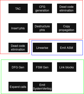
• red: Shared stages
• blue: x86-64 backend stages
• green: HardWACC stages

The pipeline starts when we move from our final AST to three-address code via TAC generation.

The CFG

Our CFG ADT was, like the AST, phased. We assigned a phase phantom type to each of the backend stages. This phase gives us two things:

• The ability to enforce ordering of operations on the CFG at a type level
• The ability to change what data is stored at each stage. In this case it was: whether the AST could have ‘undefined’ values inside instructions; what data was stored in the phis field.

// BodyInstruction <: Instruction
// TerminatorInstruction <: Instruction
final case class Block[P <: Phase](
    body: List[BodyInstruction[DefinednessOf[P]]],
    terminator: TerminatorInstruction[DefinednessOf[P]],
    phis: PhisOf[P] = ()
)

final case class CFG[P <: Phase](
    params: List[Var],
    entry: Label,
    blocks: TreeMap[Label, Block[P]]
);

The code composing our stages looked like this:

  val verilog = tacgen
    .generate(program, config)
    .generateCfg
    .simplify
    .insertPhiDestinations
    .insertPhis
    .destructurePhis
    .copyCleanup
    .removeUselessAssigns
    .makeDfgs
    .genFSM
    .toDoc
    .render

SSA

We implemented SSA with these stages:

• Dominator tree creation (Cooper et al.)
• Dominance frontier creation (Cytron et al.)
• Renaming (Cytron et al.)
• Breaking critical edges
• Replace phis with parallel copies

HardWACC

HardWACC is a high-level synthesis tool for WACC which compiles to SystemVerilog, made in roughly 1 week. The source WACC program is translated into a finite state machine that can be synthesised onto an FPGA or an ASIC (we tested on an FPGA). HardWACC obviously has many performance advantages over regular WACC as the hardware is specialised for executing the WACC program, including parallelising as many instructions as possible within each clock cycle.

We used an Intel DE10-Lite board for testing so we added a few board-specific features, such as displaying the exit code of the program on the board’s seven-segment display.

For HardWACC, we had to remove a few features from the WACC language, notably dynamic memory allocation, due to practical reasons and time constraints. HardWACC can still compile most other WACC programs and there are still many interesting points of discussion regarding how it works.

Compilation pipeline overview

The whole front-end, and some mid-end, of the compiler remains the same: parsing, typechecking, SSA construction etc. The HardWACC compilation process branches off the regular compilation process after the phi-destruction stage, so compiling to SystemVerilog begins with a CFG in SSA form without any phis.

From here, each CFG basic-block is replaced with a dataflow graph (DFG), where each instruction is a node and its edges connect to the instructions that are the dependencies of the instruction. Take this block for example:

t1 = 1 + 1
t2 = t1 * 2
t3 = t1 / 3

The nodes representing the definition of t2 and t3 will both have an edge connecting to t1, as defining t1 is a requirement to define t2 and t3.

With a CFG full of DFGs, we can start ASAP scheduling. The cycle number of an instruction is just 1 + the max cycle number of all of its dependencies, given that every operation takes a single cycle. Constants and variables defined outside the current block are obviously available from cycle 0. So for the above snippet, t1 will execute on cycle 1 and t2 and t3 will execute on cycle 2.

val cycleMap = mutable.Map.empty[NodeId, StateId]

def calcState(nodeId: NodeId): StateId = {
  dfg.nodes(nodeId) match {
    case Node.BinOp(_, left, right) =>
      max(cycleMap(left), cycleMap(right)) + 1
    
    // Node.Identity is a raw assignment i.e t2 = t1
    case Node.Identity(right) => cycleMap(right) + 1
    
    // the remaining are always available 
    case Node.Const(_, _)     => 0
    case Node.Data(_)         => 0
    // Node.Input refers to a variable that is used in the block
    // but defined outside of it
    case Node.Input(_)        => 0
  }
}

// reverse topological sort of the DFG ensures all dependencies
// of an operation are defined in the cycle map before
// processing that operation
dfg.getReverseTopologicalSort().foreach { nodeId =>
  cycleMap += nodeId -> calcState(nodeId)
}

It’s also easy to make the cycle number unique across the entire program, which makes up the bulk of the finite state machine. Jumps and branches also map nicely to state transitions, although at this stage these jumps are likely just to labels. In a subsequent pass over the FSM, called the link blocks phase, we replace all labels with the state number they correspond to.

Lastly, we print the SystemVerilog program directly from the FSM, which paired with our own SystemVerilog modules gives us a complete WACC program description in hardware. We have one state register storing the current state, as well as one register for each temporary variable that is used in the program. On each positive clock edge, the register assignments corresponding to the current state, as well as updating the state register to the next state are all executed simultaneously.

typedef enum logic [6:0] {
        S0 = 7'd0,
        S1 = 7'd1,
        S2 = 7'd2,
        // ...
} state_t;

state_t state;

logic [31:0] r1 = 32'd0;
logic [31:0] r2 = 32'd0;
logic [31:0] r3 = 32'd0;
// ...

always_ff @(posedge CLOCK_50) begin
    case (state)
        S1: begin
            r1 <= 1 + 1;
            state <= S2;
        end
        S2: begin
            r2 = r1 * 2;
            r3 = r1 / 3;
            state <= S3;
        end
        S3: begin
            // ... 

When the program terminates, it sets two output registers of the program: a 32-bit register containing the exit code and a “done” bit signalling the end of the program. When “done” is set to 1, we display the exit code on the seven-segment display with the help of some of our own SystemVerilog modules.

Of course, this is a massive oversimplification of the whole compilation pipeline, and doesn’t touch on the issues introduced by features like console output and function calls. Let’s get into the details :D

Function calls

Block splitting

Each CFG block gets translated to a DFG, which is then used to schedule individual instructions. Typically, control-flow instructions like jumps and branches are terminating instructions that do not occur within the body of a block, simply mapping to a state transition that is scheduled after all of the body instructions are executed. Function calls however are not terminating instructions, and occurs as a body instruction. This is problematic when it comes to scheduling. Take the following block for example:

t1 = 1 + 1
t2 = t1 - 3
t3 = call f(t1)
t4 = t3 * 7

How would we go about scheduling this? It’s obvious that t1 is assigned to cycle 1 and t2 is assigned to cycle 2, but what cycle is t3 or t4 assigned to? We have to wait however many cycles it takes for the function f to run before assigning to t3 or t4, but we don’t know how many cycles that will be because statically determining the exact cycle count of an arbitrary function is undecidable in the general case.

Our solution is to split the CFG block in two at the call site:

Block 1:

t1 = 1 + 1
t2 = t1 - 3

Block 2:

t4 = t3 * 7

We have to do two things when making the split:

1. Make block 1’s block transition be a Call, which contains the callee name f, the list of arguments (t1) and a reference to block 2 as the location to resume execution.
2. Mark on block 2 that it should retrieve the function’s return value and store it in t3 immediately. This assignment will get added when generating the FSM and will be scheduled for the first cycle in this new block.

Splitting the block moves the complexity of function calling to state transitions rather than dealing with them as individual instructions, which is great because now we can schedule block 1 and block 2 independently.

FSM call expansion

When we call a function in a finite state machine, what should happen? The first most obvious thing is we should transition to the state that’s at the start of the function. Passing arguments is as simple as directly writing to every register the function uses as a parameter. However, overwriting all of a function’s registers is problematic if we want to add recursion to the language, as if a function calls itself, once the caller resumes execution, all of the registers will be clobbered. This means we need a call stack that pushes the current function’s registers (if we are calling ourself), as well the state to return to. That state to return to should then be the start of the sequence of pops of the registers from the stack back to their correct registers, before resuming normal execution.

All of the above happens in the call expansion phase. This is the final FSM transformation, which replaces all Call state transitions with the

push args -> call function and save return state -> pop args -> resume

state sequence.

Stack implementation

The stack is implemented in SystemVerilog as a large array, which gets synthesised to on-chip BRAM. The stack is of fixed-width (32 bits) as BRAM ports are configured to a fixed data width at synthesis time; the width is physically baked into the memory block’s address decoding and cannot vary at runtime. This means pushing an 8-bit boolean to the stack requires padding an extra 24 bits to fit the stack width, which might seem like a waste, but it keeps the read, write and stack pointer logic simple.

IO

HardWACC provides a UART interface for IO (well, O). We bundle a UART interface module in the generated code, along with a print buffer module that abstracts the usage to make it make the actual FSM simpler to generate.

Our clock rate is 50MHz, and our baud rate is 115200Bd (we transmit one bit at a time, so 115200b/s). This means each bit takes 434 clock cycles to transmit. Printing is very slow, as expected.

HardWACC improvements for the future

Having completed the project in such a short timespan, there’s a lot that can be done to improve the generated SystemVerilog.

Firstly is register allocation. Right now we have a one-to-one register mapping from the infinite-register IR to SystemVerilog, as there isn’t a hard limit on the number of registers like on typical CPU architectures. This does waste area however, and it would be nice if we could use liveness analysis to bundle multiple registers together where possible. This paper on register allocating SSA programs might be a good starting point, as we would be able to have optimal interference graph colouring in polynomial time (no heuristic colouring), without the pain points of spilling as we can choose the number of available registers.

Another improvement would be in how we schedule instructions. Currently, intermediate instructions in a computation each have their own state in the FSM, even if the final result is purely combinational. What we could do is fit all of these instructions into the same cycle if the propagation delay of the circuit fits in a clock period.

The WACC language supports user input, which we did not have time to implement. This would be something to consider for the future. Adding a receiver to the UART interface wouldn’t be so hard, but how that interacts with our FSM could be an interesting challenge.